Scene
Built to accompany our report on Causality in Machine Learning, Scene shows how we applied the invariant risk minimization (IRM) technique to a portion of the iWildcam dataset.
With IRM, you group training data into environments. Being explicit about environments helps minimize spurious correlations during model training. Below, we guide you through the process and model results using images from the dataset.
Contents
Training environments
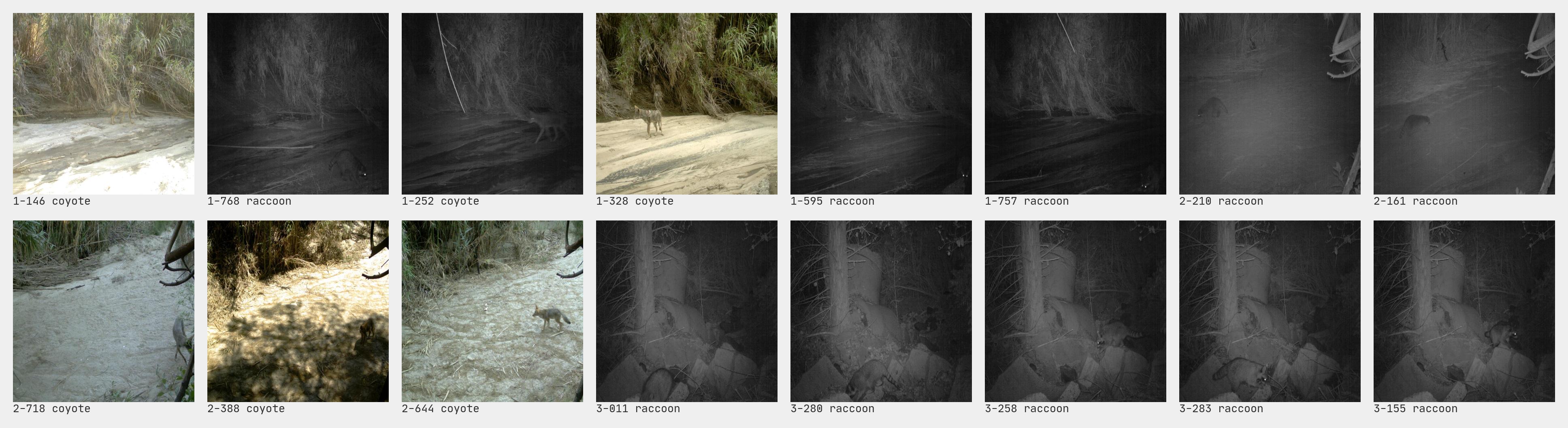
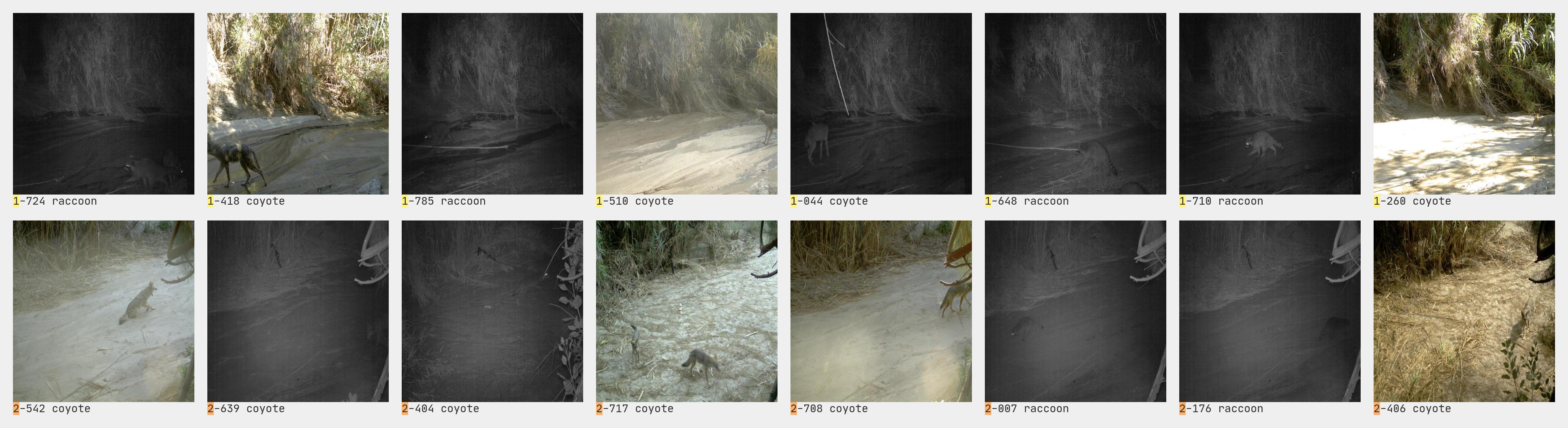
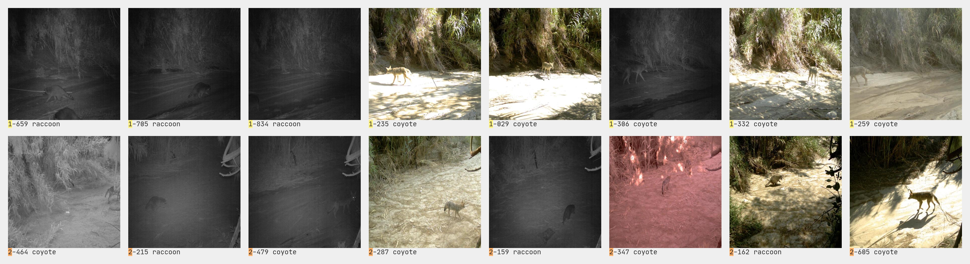
We trained a binary classifier, so we further limited the dataset to images of coyotes and raccoons. The final numbers for our training datasets are:
- environment 1
- 858 images
- 582 coyotes
- 276 raccoons
- 858 images
- environment 2
- 753 images
- 512 coyotes
- 241 raccoons
- 753 images
Model training
Results: training dataset
Now let's take a look at how our trained models performed. On the combined training datasets (1 & 2) their accuracy is nearly equal. As a baseline, a model that always predicted coyote would achieve 68% accuracy (because the majority of the images in the dataset are coyotes).

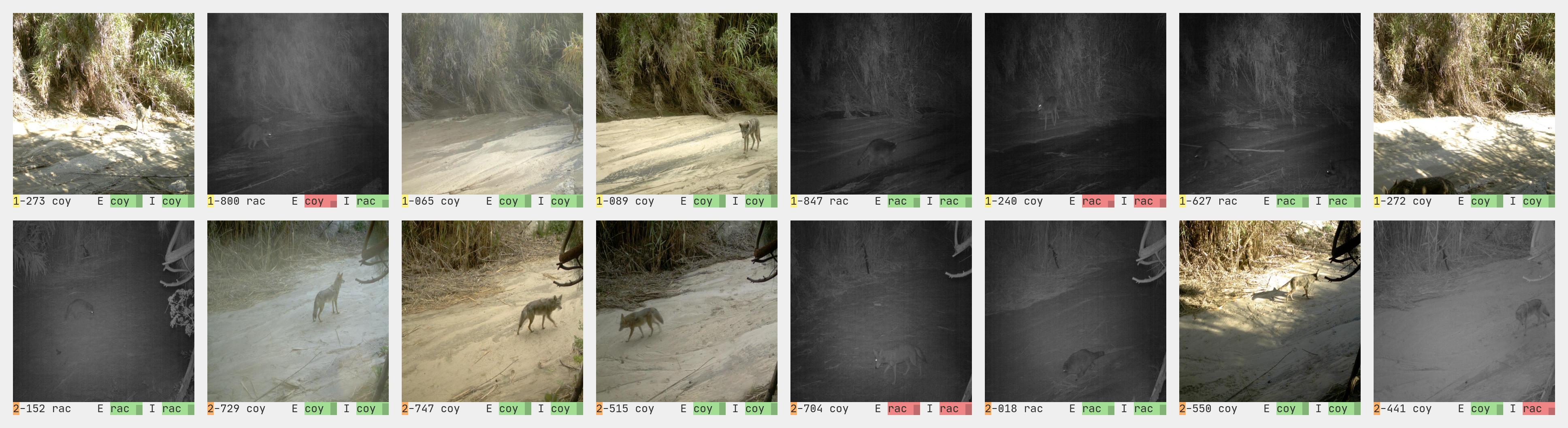
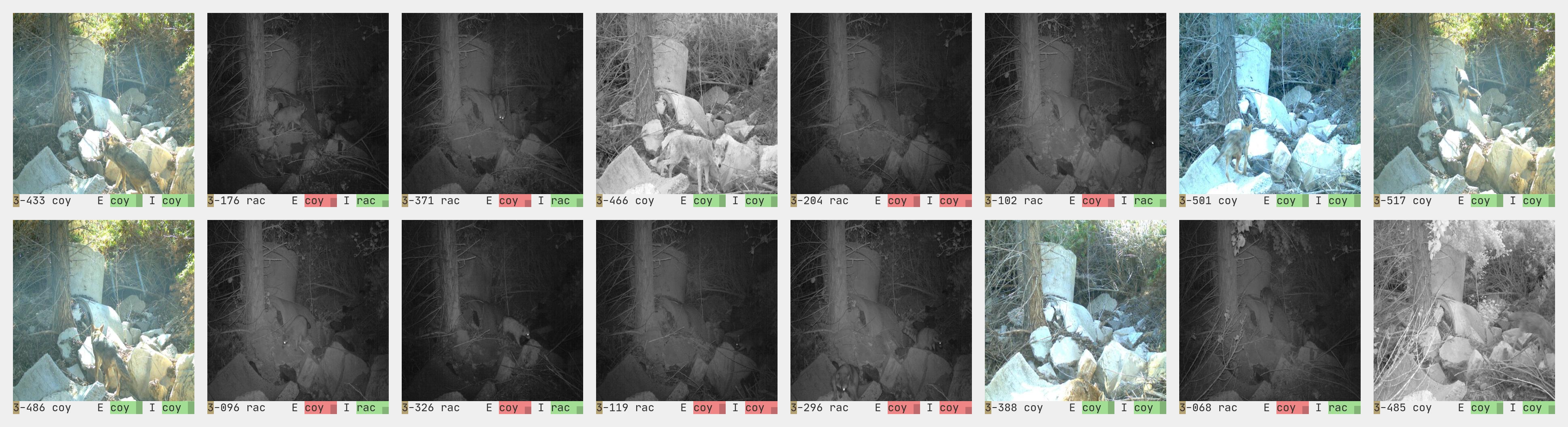
Reading the classifications
Results: test dataset
But now look at what happens when we introduce a third environment:

For our test dataset, environment 3, we used a different camera from the iWildcam dataset, which neither model saw during training. On the new dataset IRM vastly outperforms ERM, with IRM achieving 79% accuracy versus the ERM model's 36%. This performance suggests IRM has made the model more accurate across different environments.
- environment 3
- 522 images
- 144 coyotes
- 378 raccoons
- 522 images
Interpretability
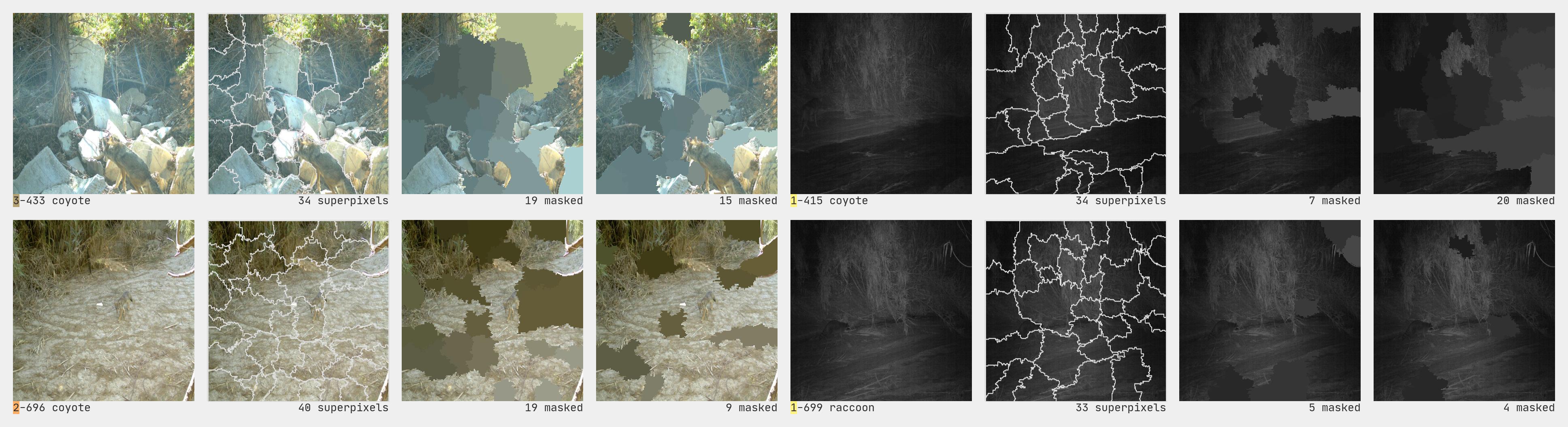
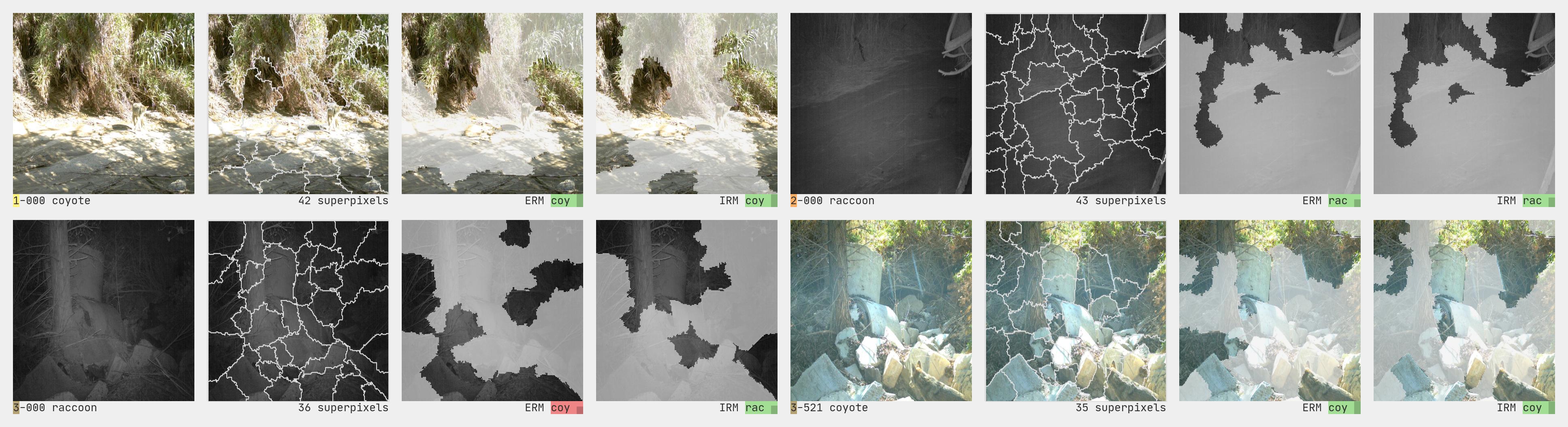
To try and better understand the models we used an interpretability technique called LIME to to visualize which parts of the image were driving the classification. To do this, LIME first splits an image into superpixels. It then creates permutations of the original image by randomly masking different combinations of those superpixels. It builds a regression model on those permutations and uses that to determine which superpixels contribute most to the classification.
Ranking superpixels
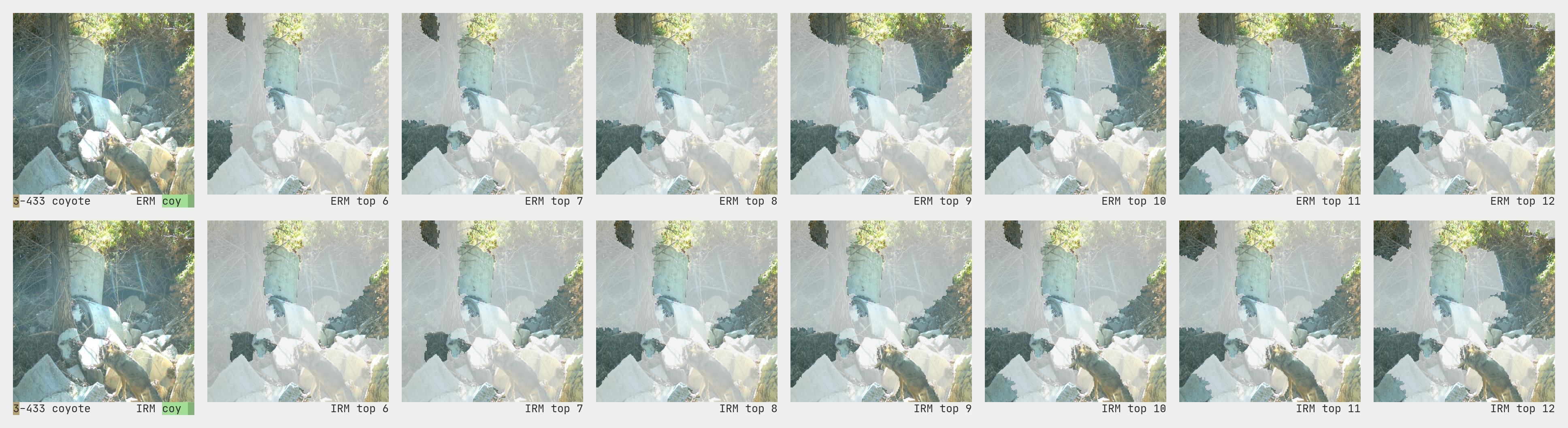
This result would seem to indicate that the IRM model is better able to focus on the invariant features (the animal) versus the variant (the background environment). That could be the explanation for why it performs better on the environment 3 dataset, which neither model has seen before.
Model comparison
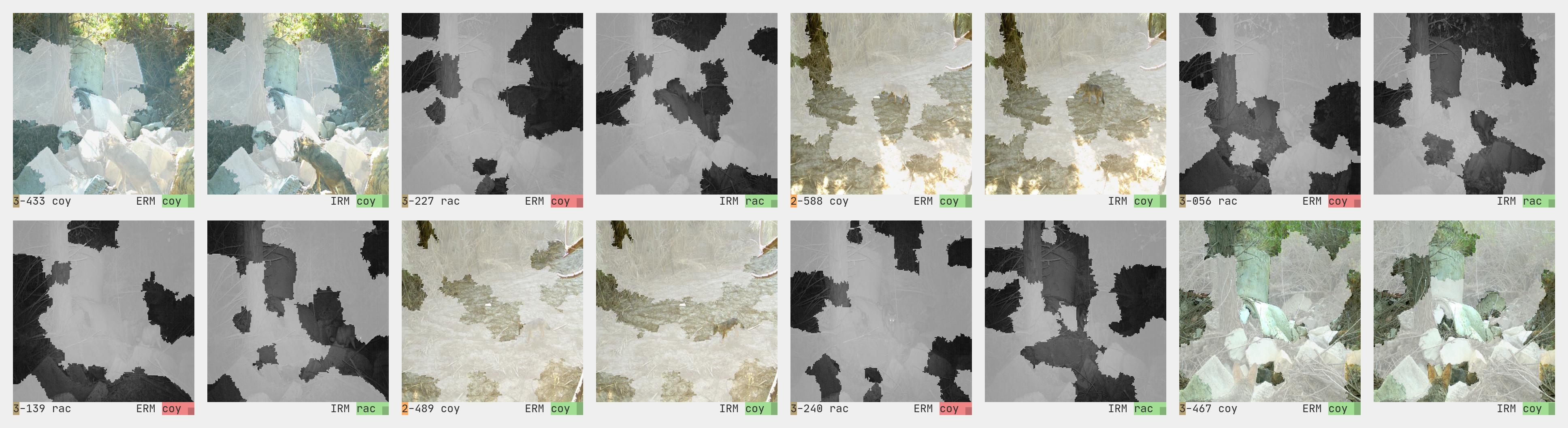
If all the of the model comparison looked like example 3-433, we could confidently say the IRM model is better at recognizing the animal across environments. 3-433 is only one example, however, and while it is definitely possible to find other images where the IRM highlighted features include the animal and the ERM do not (as in the examples shown here, where the top 12 features for each model are highlighted) it is definitely not the case for all of the images.
Looking through the entire dataset reveals a lot of variation in which superpixels are highlighted for each model. The lack of a consistent, obvious pattern in the top features could mean neither model is successfully isolating the animal features, or it could mean this interpretability approach is not capable of visually capturing their focus. It could also be both.
See more
For more discussion on how we approached building these models, read the prototype section of our report. The larger report puts IRM in the context of the larger efforts to bring causality into machine learning.